1. Intro

In recent years, there has been growing interest in using multiregional social accounting matrix (SAM) models. These models require reliable estimates of inter-regional trade. Because detailed data on the commodity-specific trade between counties are not available, several estimation techniques have been used.

The methods used to estimate the interregional trade flows can substantially affect both the interregional multipliers and the estimated impacts that are derived from multiregional SAM models (Robison and Liu, 2006).

In 2005, IMPLAN Group (formerly MIG, Inc.), in concert with the U.S. Forest Service, developed a doubly-constrained gravity model to estimate trade flows for all IMPLAN commodities between all counties in the U.S. This trade flow model serves several purposes, including the following:

It is used to calculate improved regional purchase coefficients (RPCs) for single-region modeling. An RPC describes the proportion of each dollar of local demand for a given commodity that is purchased from local producers, with higher RPCs indicating less leakage and larger input-output (I-O) multipliers. Prior to development of the trade flow model, IMPLAN Group used a set of econometric equations to estimate RPCs for each shippable commodity (Alward and Despotakis, 1988). The econometric equations were derived from a 51-region, 120-industry multi-regional input-output (MRIO) model developed by Jack Faucett Associates, Inc. (1983). This work was based on 1977 data and represents an update of pioneering MRIO work done by Polenske (1970). The RPCs for non-shippable commodities (i.e., services) were based on the “observed” values from a 51-region MRIO created by Havens (xxxx) based on 1982 data. The econometric RPC methodology has yet to be updated and as a statistical approach it is susceptible to the estimation error associated with statistical analysis.

1. It is used to make possible MRIO modeling with the IMPLAN software, thereby allowing the user to view indirect and induced impacts on regions other than the base region where the direct impact occurs.
2. It serves as the basis for developing multi-regional SAM models that can be incorporated into other software.
3. This paper discusses the development of IMPLAN’s trade flow model.

2. The Gravity Model

2.1. The Gravity Model Form

The gravity model was originally adapted from Newton’s Law of Gravity, which states that the attraction between two masses is directly related to the size of the masses and inversely related to the distance between them:

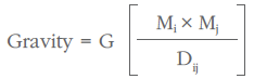
where G is a constant representing the force of gravity.

The gravity model was first suggested in an I-O context in Leontief and Strout (1963). In the last fifty years, the gravity model has been widely — and effectively — used to predict trade flows (Federal Highway Administration, 1977, p. 118; Anderson and van Wincoop, 2003; Anderson, 2011). In this context, gross supply and demand often serve as the mass variables. If the effect of distance is ignored, we may expect that, for a given commodity, the proportion of supply of that commodity going from region i to satisfy demand in region j will be equal to the ratio:

where D_j = region j’s total demand for the commodity and D = total demand for the commodity across all regions. For example, if region j makes up 10% of total domestic demand for the commodity, then each region that produces the commodity will send 10% of its domestic supply of that commodity to region j. The greater the proportion of domestic demand for the commodity that stems from region j, the greater will be the proportion domestic supply of the commodity that flows to region j.

In this case, trade between regions i and j depends solely upon supply and demand in each region — supply from region i will go to meet the demand in region j based on region i’s total production of the commodity and region j’s proportion of all regions’ demand for the commodity:

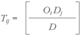
where T_ij = trade flows of the commodity from region i to region j and O_i = total supply of the commodity originating in region i.

However, distance can have a countervailing effect on trade. Given the size of region j, the amount of trade flows from region i to region j will decrease as the distance between regions i and j increases. This situation can be described as follows:

and

where d_ij is the distance between regions i and j). It has been shown that the effect of distance on trade is not uniform (Isard, 1960; Carol and Bevis, 1957). The solution suggested by empirical studies is to raise the distance variable to some exponent b, thereby giving large distances a greater proportional deterrence than small distances. The question of what value to give to the exponent b is a difficult one that is decided during the calibration of the model; this will be discussed in section 4.2.

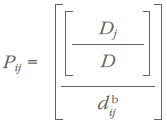
It will simplify the process if we re-write equations 4 and 5 as follows:

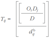
and

Experience has shown that Equations 6 and 7 overestimate the volume of shorter hauls (Isard, 1960; Carroll and Bevis, 1957). This led to reformulation of the gravity model to account for all competing sources of demand:

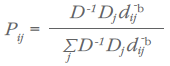
and

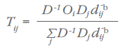
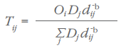
We can simplify equations 8 and 9 by recognizing that D^-1 can be pulled out of the summation since it is constant for all regions. The D^-1 then cancel out:

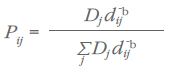
and

We can simplify further by setting:

Therefore:

and

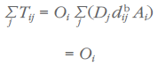
Because the sum of all probabilities (P_ij s) is 1, we can derive a singly-constrained model where the sum of all trade from region i to all regions is equal to the total supply in region i:

But we also need to constrain the system so that the sum of all trade flows into region j is equal to that region’s total demand. The known D_j is divided by the estimated total inflows, yielding the ratio:

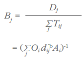
Each first-round supply-constrained estimate of T_ij to destination j is then multiplied by B_j to obtain the first round of demand-constrained estimates of T_ij:

For each origin region i, the known O_i is then divided by the new demand-constrained estimates of ∑_i T_ij , yielding the ratio:

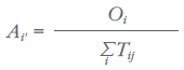
Each demand-constrained T_ij for origin i is then multiplied by A_i' to obtain the next round of supply-constrained estimates of T_ij:

This iterative process is repeated until the trade estimates are double-constrained; that is, until all supplies go somewhere (including within the same county) and all demands are fulfilled. When the computation comes to an end, each trade flow will have been multiplied in succession by one or more ratio A_i, A_i', A_i'',… and one or more ratio B_j, B_j', B_j'',… Equation [19] then becomes:

where A_i = A_i × A_i' × A_i''… and B_j = B_j × B_j' × B_j''… A_iB_j may be thought of as a derived gravitational constant reflecting the complementarity of the attributes of the two regions (Isard, 1998, p. 262). This formulation assures that the following two constraints are satisfied:

and

2.2. Distance

In the earliest empirical tests of the gravity model, distance was used as the impedance variable. The simplest concept is the straight-line distance or shortest possible route between two regions. This route can be determined through GIS programs and is known as the great circle distance. Once the great circle distances between regions is known, a simple rule-of-thumb could be used to estimate highway distance between regions — e.g., the highway distance between regions i and j is 1.2 times the gcd between regions i and j.

It is apparent, however, that pure distance is not a sufficiently accurate measure of the effects of spatial separation (Lee, 1973, p. 69). Neither of the above approaches accounts for the relative advantages of rail and water transportation, nor impediments to travel. For example, the great circle distance or highway distance between Denver and New Orleans may be shorter than the highway distance between St. Paul and New Orleans, but water transportation available on the Mississippi River means that grain shipments are more likely to travel from St. Paul to New Orleans than from Denver to New Orleans.

Wilson (1969) suggests that the most relevant variable is cost. Indeed, distance is frequently equated with the cost of moving goods and services from one location to another. The Center for Transportation Analysis at Oak Ridge National Laboratory (ORNL) has developed an integrated, intermodal transportation network modeling system. The system accounts for tolls, congestion, and other factors to derive travel impedances between each county centroid to every other county centroid in the U.S. by mode of transportation (truck, truck-rail multimodal, and truck-water multimodal). Weighted averages of these impedances (based on a commodity’s modal mix as reported by the Commodity Flow Survey) serve as the distances (d_ij) in IMPLAN’s gravity model. ORNL also provides us the great circle distances between county centroids — these are used to calibrate the gravity model to Commodity Flow Survey data, as described next.

2.3. Model Calibration

The Commodity Flow Survey (CFS) and Freight Analysis Framework (FAF) contain information on the value, weight, distance traveled, transportation mode, and origin and destination state of the shippable commodities. These commodities are classified according to the standard classification of transported goods (SCTG) system, and the survey data are typically reported at the two-digit SCTG level. The tables from the CFS and FAF provide three important pieces of information relevant to the gravity model:

1. Mode of transportation by commodity
2. Tons by distance shipped
3. Ton-miles shipped

Mode of Transportation

CFS and FAF tables show the proportion of total commodity value, tons, and ton-miles that were transported by the various transportation modes. This table of shipment mode provides the basis of our decision as to which of the impedances to use in calibration of the model or the weighting to give the various modes of transportation.

Ton-Miles

Finally, after determining the appropriate value and functional form for dij, perhaps the most important part of the calibration is determining an appropriate value for b. For this we rely on CFS and FAF data on value, tons, and total ton-miles moved by commodity. Dividing ton-miles by tons for a commodity yields the average movement for each ton of that commodity, which serves as the target for calibration — b is adjusted for each commodity until the sum of Tijs for that commodity (for all i and j) are suitably close to the national average movement of that commodity as reported by the most recent CFS.

The calibration process begins by setting b to a value of 2 (the value of b in Newton’s gravity formulation) and solving the doubly-constrained model for initial estimates. If the average ton-miles exceeds the target from the calibration sources, b is increased, thereby decreasing the “distance” between i and j. Conversely, if the average ton-miles is less than the target value, b is decreased. This is done iteratively until the average ton-miles traveled by the commodity (across all counties) is within ten percent of what the calibration sources report as the national average movement of that commodity.

3. Implementation in IMPLAN

Each year, the IMPLAN database is used to create the attracting masses (supply and demand) for each U.S. county. Impedances are then derived from ORNL’s Transportation Network model between centroids for all U.S. counties to represent distances between the masses. The most recent CFS is then used to calibrate the gravity model. Even with this tremendous and unique collection of data, a number of assumptions are necessary for the trade flow model to work, including the following:

1. A fully defined gravity model can estimate trade flows between counties.
2. The 2-digit to 4-digit SCTG data from the CFS can be bridged to the 300-plus IMPLAN manufactured commodities without a sacrifice in accuracy or loss of critical information in aggregation.
3. The CFS average ton-miles moved is a good indicator of the average distance commodities travel from point of production to point of consumption.
4. A satisfactory b value can be derived for the service sectors. Without CFS data for calibration, this is a more subjective process.

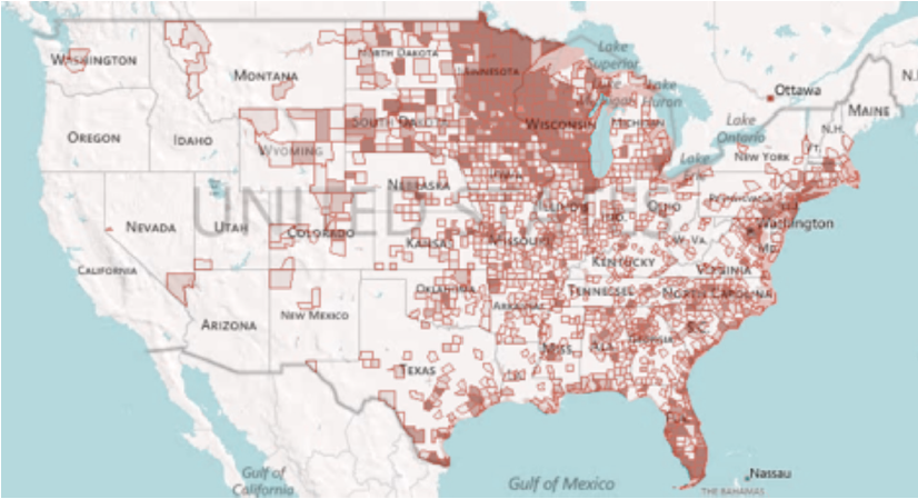
Although there is no way to definitively prove that the trade flows are correct, one way to examine the reasonableness of the flows is to map them. Figure 1 shows the flow of fluid milk and butter from St. Croix County, WI to the rest of the U.S. In Figure 1, there is a wide scattering of points, but the color of the points is relative, with darker colors representing greater shipment values. The model is allocating some supply to a large number of counties. What is interesting here is the relative lack of shipments to the Western half of the U.S. as well as the New England states. California is the number one supplier of raw milk in the U.S. and has a lot of processing. In New England, there is a contract that supports the milk industry and shuts out most other suppliers. Thus, it is a good sign that the trade flow model shows relatively few flows to these regions. The inter-county trade data can be summed to determine the trade between any grouping of counties or states and any other grouping of counties or states.

Figure 1. Fluid Milk and Butter Shipments from St. Croix County, WI

4. Limitations and Opportunities

The CFS data report shipment origin rather than manufacturing origin, which can underestimate the average ton-miles moved for commodities that are held in warehouses prior to being shipped to the demanding industry or institution.

The CFS covers shippable commodities only; there is no inventory of trade flows for services. Thus, there is currently no calibration process for service flows; the b’s are selected based on analyst judgment. While commuting data could potentially provide an estimate or the average distance traveled by consumers to obtain services, we would also need the value of services per trip or per mile. A further complication is that individuals also consume services when traveling longer distances (i.e., for business and pleasure) than their typical day-to-day travels. Jackson (2002) used averages from the manufacturing sectors under the assumption that interregional trade in these sectors is related to information flows, which as the authors assert should be reflected by patterns of overall trade. Realistically, it should be expected that manufactured goods, on average, would travel much farther than consumers would be willing to travel to receive a service. On the other end of the spectrum, Park et al. (2007) assumed no inter-state flows of services as a preferred alternative to unreliable estimates.

One criticism of gravity models is that while they may describe interaction patterns satisfactorily, they do not explain them. Nonetheless, while the simple structure — with few parameters — of the gravity model does not identify the complex chain of cause and effect which gives rise to the trade patterns, the patterns described by the model can reasonably be expected to remain more or less stable over the short (and perhaps medium) term (Lee, 1973, p. 67). The variables supply, demand, and distance (the last of which is itself a function of travel time and cost) capture, in a sense, the explanatory power of many of those unobserved factors because they themselves are the result of those factors.

While it is theoretically possible to model foreign markets as additional regions, IMPLAN does not currently do so. Thus, the gravity model is based solely on domestic supplies and demands — foreign imports and exports are removed from the model a priori.

References

Alward, G.S. and K. Despotakis. 1982. “IMPLAN Version 2.0: Data reduction Methods for Constructing Regional Economic Accounts”. Paper. USDA Forest Service, Fort Collins, CO.

Alward, G., D. Olson, and S. Lindall. 1998. Using a Double—Constrained Gravity Model to Derive Regional Purchase Coefficients. Paper delivered at the 45th North American Meetings of the Regional Science Association International. Santa Fe, NM: November 11-14, 1998.

Anderson, J.E. and E. van Wincoop. 2003. Gravity with Gravitas: A Solution to the Border Puzzle. The American Economic Review, 93(1): 170-192, March.

Anderson, J.E. 2011. The Gravity Model. Annual Review of Economics, Volume 3: 133-160.

Ando, A. and T. Shibata. 1997. A Multi-Regional Model for China Based on Price and Quantity Equilibrium. In M. Chatterji (ed.), Regional Science: Perspectives for the Future, New York, NY: St. Martin’s Press, Inc.

Brown, H.J., J.R. Ginn, and F.J. James. 1972. Land-Use-Transportation Planning Studies. In Brown, H.J., J.R. Ginn, F.J. James, J.F. Kain, and M.R. Straszheim (eds.), Empirical Models of Urban Land Use: Suggestions on Research Objectives and Organization, National Bureau of Economic Research, www.nber.org/books/brow72-1, last accessed June 2011.

Carroll, J.D. and H.W. Bevis. 1957. Predicting Local Travel in Urban Regions. Papers and proceedings of the Regional Science Association, Vol. 3.

Federal Highway Administration. 1977. Computer Programs for Urban Transportation Planning.

April, http://www.otdmug.org/resources/planpacbacpac-general-information.aspx, last accessed May 2012.

Gómez Herrera, E. 2010. Comparing Alternative Methods to Estimate Gravity Models of Bilateral Trade. The Papers 10/05, Department of Economic Theory and Economic History of the University of Granada.

Harris, B. 2001. Accessibility: Concepts and Applications. Journal of Transportation and Statistics, Vol. 4, No. 2/3, http://www.bts.gov/publications/journal_of_transportation_and_statistics/volume_04_number_23/paper_02/index.html, last accessed March 2012.

Havens, John. xxxx

Isard, W. 1960. Methods of Regional Analysis. MIT Press.

Isard, W. 1998. Gravity and Spatial Interaction Models. In W. Isard, I.J. Azis, M.P. Drennan, R.E. Miller, S. Saltzman, and E. Thorbecke (eds.), Methods of Interregional and Regional Analysis, Brookfield: Ashgate.

Jack Faucett Associates. 1983. “The Multiregional Input-Output Account, 1977”; Vols. I-IV; Report submitted to the US Department of Health and Human Services, Contract #HHS-100-81-00-57, July.

Jackson, Randall W. 2002. Constructing US Interregional SAMs from IMPLAN Data: Issues and Methods. 2002-14. Morgantown, WV: Regional Research Institute, West Virginia University.

Lee, C. 1973. Models in Planning: An Introduction to the Use of Quantitative Models in Planning. Pergamon Press.

Leontief, W. and A. Strout. 1963. “Multiregional Input-Output Analysis.” In T. Barna (ed.), Structural Interdependence and Economic Development, London: Macmillan (St. Martin’s Press), pp. 119-149.

Miller, R.E. and P.D. Blair. 2009. Input-Output Analysis: Foundations and Extensions. New York, NY: Cambridge University Press.

Park, J.Y. 2006. Estimation of State-by-State Trade Flows for Service Industries. Paper presented at the North American Meetings of the Regional Science Association International 53rd Annual Conference, Toronto, Canada, November 16-18, 2006.

Park, J.Y., P. Gordon, J.E. Moore II, and H.W. Richardson. 2007. Simulating the State-by-State Effects of Terrorist Attacks on Three Major U.S. Ports: Applying NIEMO (National Interstate Economic Model). In H.W. Richardson, P. Gordon, and J.E. Moore II (eds), The Economic Costs and Consequences of Terrorism. Cheltenham: Edward Elgar, 208-234.

Polenske, Karen R. 1970. “A Multiregional Input-Output Model for the United States”. EDA Report No. 21 (Harvard Economic Research Project). Revised December 1970.

Tolbert, C.M. and M. Sizer. 1996. “U.S. Commuting Zones and Labor Market Areas: A 1990 Update”. Staff Paper #AGES -9614. Rural Economic Division, Economic Research Service. U.S. Department of Agriculture.

U.S. Department of Transportation and U.S. Department of Commerce. 1999. 1997 Commodity Flow Survey.

U.S. Department of Transportation Bureau of Transportation Statistics and U.S. Census Bureau Economics and Statistics Administration. 1999. Publication EC97TCF-US, December.

Wilson, A.G. 1969. Entropy in Urban and Regional Modeling. Centre for Environmental Studies, Working Paper 26.